[DL] 딥러닝 개요 - 기초 모델

딥러닝이란?

인간의 뉴런이 학습하는 방식을 모사하여 만든 기계 학습 방법이다.

출처 : 네이버 블로그 LEE&JANG ECO

 

 

예제 코드를 보며 그때그때 필요한 설명을 덧붙일 것이다.

 

---

 

[ XOR 분류 ]

 

1. 먼저 필요한 라이브러리를 모두 import 한다.

import tensorflow as tf
import tensorflow_datasets as tfds
import numpy as np
import pandas as pd
import matplotlib.pyplot as plt
from IPython.display import Image
import os, shutil

 

 

2. 데이터 생성 및 확인

# random data 생성
tf.random.set_seed(1)
np.random.seed(1)

# data 조건 지정
x = np.random.uniform(low=-1, high=1, size=(200, 2))
y = np.ones(len(x))
y[x[:, 0] * x[:, 1]<0] = 0

# train, valid data 분할
x_train = x[:100, :]
y_train = y[:100]
x_valid = x[100:, :]
y_valid = y[100:]

# 데이터 plot
fig = plt.figure(figsize=(6, 6))
plt.plot(x[y==0, 0], 
         x[y==0, 1], 'o', alpha=0.75, markersize=10)
plt.plot(x[y==1, 0], 
         x[y==1, 1], '<', alpha=0.75, markersize=10)
plt.xlabel(r'$x_1$', size=15)
plt.ylabel(r'$x_2$', size=15)
plt.show()

위 데이터를 나누는 것이 목표이다.

 

---

 

★★ 3. 딥러닝 모델 설정 및 학습 - 단층 퍼셉트론 ★★

 

이 과정은 아래 3단계로 이루어진다.

모델 쌓기 → 컴파일(compile) → 모델 학습(fit)

 

#모델 설정 - 단층 퍼셉트론
model = tf.keras.Sequential()
model.add(tf.keras.layers.Dense(units=1, 
                                input_shape=(2,), 
                                activation='sigmoid'))

model.summary()

먼저 Sequential을 기본으로 놓고, 그 위에 layer를 add하는 방식으로 모델을 build한다.

예제에서 사용된 Dense layer의 파라미터들의 기능은 아래와 같다.

Parameter	기능
units	출력 데이터의 차원 수
input_shape	입력 데이터의 형태
activation	활성화함수

* 활성화 함수의 종류 *

활성화 함수(Activation Function)	설명
relu	{ 0 , Z }
leakyrelu	{ -0.01, Z }
tanh	{ -1, 1 }
sigmoid	{ 0, 1 } 범주형 결과가 두개인 경우
softmax	범주형 결과가 두개 이상인 경우

 

#모델 컴파일
model.compile(optimizer='SGD',
              loss='BinaryCrossentropy',
              metrics=['BinaryAccuracy'])

#모델 학습
hist = model.fit(x_train, y_train, 
                 validation_data=(x_valid, y_valid), 
                 epochs=100, batch_size=2)

* 모델 컴파일 *

Parameter	기능	종류
optimizer	경사하강법	SGD, adam 등
loss	오차	BinaryCrossentropy, CategoricalCrossentropty
metrics	모델 평가 방법(정확도)	Accuracy, BinaryAccuracy, CategoricalAccuracy 등

 

---

 

★★ 4. 결과 확인 - 단층 퍼셉트론 ★★

 

#결과 확인
from mlxtend.plotting import plot_decision_regions

history = hist.history

fig = plt.figure(figsize=(16, 4))
ax = fig.add_subplot(1, 3, 1)
plt.plot(history['loss'], lw=4)
plt.plot(history['val_loss'], lw=4)
plt.legend(['Train loss', 'Validation loss'], fontsize=15)
ax.set_xlabel('Epochs', size=15)

ax = fig.add_subplot(1, 3, 2)
plt.plot(history['binary_accuracy'], lw=4)
plt.plot(history['val_binary_accuracy'], lw=4)
plt.legend(['Train Acc.', 'Validation Acc.'], fontsize=15)
ax.set_xlabel('Epochs', size=15)

ax = fig.add_subplot(1, 3, 3)
plot_decision_regions(X=x_valid, y=y_valid.astype(np.integer),
                      clf=model)
ax.set_xlabel(r'$x_1$', size=15)
ax.xaxis.set_label_coords(1, -0.025)
ax.set_ylabel(r'$x_2$', size=15)
ax.yaxis.set_label_coords(-0.025, 1)

plt.show()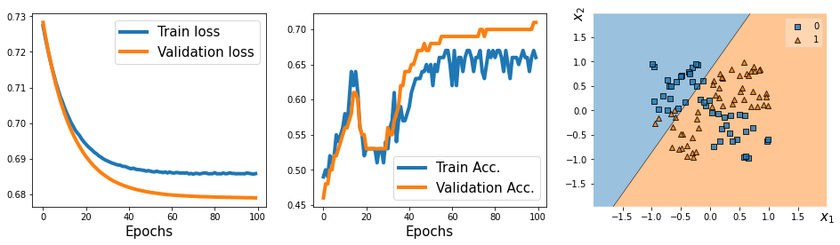

.

 

loss 는 Epoch이 반복됨에 따라 줄어들었지만, 결과적으로 분류된 경계가 0과 1을 제대로 분리했다고 볼 수 없다.

따라서, 다층 퍼셉트론으로 다시 예측해보도록 한다.

 

 

---

★★ 5. 딥러닝 모델 설정 및 학습 - 다층 퍼셉트론 ★★

# 모델 build
model = tf.keras.Sequential()
model.add(tf.keras.layers.Dense(units=4, input_shape=(2,), activation='relu'))
model.add(tf.keras.layers.Dense(units=4, activation='relu'))
model.add(tf.keras.layers.Dense(units=4, activation='relu'))
model.add(tf.keras.layers.Dense(units=1, activation='sigmoid'))

# 모델 확인
model.summary()

#모델 컴파일:
model.compile(optimizer='SGD',
              loss='BinaryCrossentropy',
              metrics=['BinaryAccuracy'])

#모델 학습:
hist = model.fit(x_train, y_train, 
                 validation_data=(x_valid, y_valid), 
                 epochs=100, batch_size=2)

 

★★ 6. 결과 확인 - 다층 퍼셉트론★★

history = hist.history

fig = plt.figure(figsize=(16, 4))
ax = fig.add_subplot(1, 3, 1)
plt.plot(history['loss'], lw=4)
plt.plot(history['val_loss'], lw=4)
plt.legend(['Train loss', 'Validation loss'], fontsize=15)
ax.set_xlabel('Epochs', size=15)

ax = fig.add_subplot(1, 3, 2)
plt.plot(history['binary_accuracy'], lw=4)
plt.plot(history['val_binary_accuracy'], lw=4)
plt.legend(['Train Acc.', 'Validation Acc.'], fontsize=15)
ax.set_xlabel('Epochs', size=15)

ax = fig.add_subplot(1, 3, 3)
plot_decision_regions(X=x_valid, y=y_valid.astype(np.integer),
                      clf=model)
ax.set_xlabel(r'$x_1$', size=15)
ax.xaxis.set_label_coords(1, -0.025)
ax.set_ylabel(r'$x_2$', size=15)
ax.yaxis.set_label_coords(-0.025, 1)

plt.show()

 

얕은 단층 퍼셉트론에 비해 다층 퍼셉트론으로 학습하고 분류 하였을 때 경계가 더 정확하다.

 

이런식으로 딥러닝 모델을 쌓고, 컴파일하고 학습시키면 된다!

모델 구조를 변경하거나, epoch/batch_size 등 파라미터들을 바꿔주면서 성능을 극대화 시키면 된다.